
Some Problems in Classical Mechanics
I. The Double Pendulum


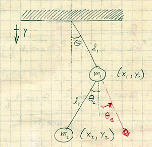
Start by writing the Cartesian coordinates in terms of polar coordinates:
| $\displaystyle{ x_1 = l_1 \sin \theta_1 = x_1(\theta_1) \text{;} }$ | (1. |
| $\displaystyle{ y_1 = l_1 \cos \theta_1 = y_1(\theta_1) }$ | (1. |
for fixed $l_1$. Likewise for the second pendulum:
| $\displaystyle{ x_2 = l_1 \sin \theta_1 + l_2 \sin \theta_2 = x_2(\theta_1, \theta_2) \text{;} }$ | (1. |
| $\displaystyle{ y_2 = l_1 \cos \theta_1 + l_2 \cos \theta_2 = y_2(\theta_1, \theta_2) }$ | (1. |
for fixed $l_1$ and $l_2$. Here it should be noted that positive $\theta_2$ is counterclockwise with the choice of positive $l_2 \sin \theta_2$ and $l_2 \cos \theta_2$. The kinetic energy with respect to the inertial reference frame is
| $\displaystyle{ T = \frac{1}{2} m_1 (\dot{x}_1^2 + \dot{y}_1^2) + \frac{1}{2} m_2 (\dot{x}_2^2 + \dot{y}_2^2) \text{,} }$ | (1. |
where
| $\displaystyle{ \dot{x_1} = \frac{\mathrm{d} x_1}{\mathrm{d} \theta_1} \dot{\theta_1} = l_1 \dot{\theta_1} \cos \theta_1 }$ | (1. |
and
| $\displaystyle{ \dot{y_1} = \frac{\mathrm{d} y_1}{\mathrm{d} \theta_1} \dot{\theta_1} = -l_1 \dot{\theta_1} \sin \theta_1 \text{.} }$ | (1. |
Furthermore,
| $\displaystyle{ \begin{align*} \dot{x_2} & = \frac{\partial x_2}{\partial \theta_1} \dot{\theta_1} + \frac{\partial x_2}{\partial \theta_2} \dot{\theta_2} + \underbrace{ \frac{\partial x_2}{\partial t} }_\text{= 0} \\ & = l_1 \dot{\theta_1} \cos \theta_1 + l_2 \dot{\theta_2} \cos \theta_2 \text{;} \end{align*} }$ | (1. |
| $\displaystyle{ \begin{align*} \dot{y_2} & = \frac{\partial y_2}{\partial \theta_1} \dot{\theta_1} + \frac{\partial y_2}{\partial \theta_2} \dot{\theta_2} + \underbrace{ \frac{\partial y_2}{\partial t} }_\text{= 0} \\ & = -l_1 \dot{\theta_1} \sin \theta_1 - l_2 \dot{\theta_2} \sin \theta_2 \text{.} \end{align*} }$ | (1. |
The potential energy with respect to the inertial reference frame is
| $\displaystyle{ V = -m_1 g y_1 - m_2 g y_2 \text{.} }$ | (1. |
The Lagrangian for the double pendulum is therefore
| $\displaystyle{ \begin{align*} L & = T - V \\ & = \frac{1}{2} m_1 (l_1 \dot{\theta_1} \cos \theta_1)^2 \\ & + \frac{1}{2} m_1 (-l_1 \dot{\theta_1} \sin \theta_1)^2 \\ & + \frac{1}{2} m_2 (l_1 \dot{\theta_1} \cos \theta_1 + l_2 \dot{\theta_2} \cos \theta_2)^2 \\ & + \frac{1}{2} m_2 (-l_1 \dot{\theta_1} \sin \theta_1 - l_2 \dot{\theta_2} \sin \theta_2)^2 \\ & + m_1 g l_1 \cos \theta_1 \\ & + m_2 g ( l_1 \cos \theta_1 + l_2 \cos \theta_2 ) \text{.} \end{align*} }$ | (1. |
Now we'll use Equation (1.11) and the Euler-Lagrange equations in the generalized coordinates $\theta_1$ and $\theta_2$:
| $\displaystyle{ \frac{\partial L}{\partial \theta_1} - \frac{\mathrm{d}}{\mathrm{d} t} \left( \frac{\partial L}{\partial \dot{\theta_1}} \right) = 0 \text{;} }$ | (1. |
| $\displaystyle{ \frac{\partial L}{\partial \theta_2} - \frac{\mathrm{d}}{\mathrm{d} t} \left( \frac{\partial L}{\partial \dot{\theta_2}} \right) = 0 }$ | (1. |
to obtain the equations of motion for the double pendulum. These are shown at Hamiltonian Chaos, where they are also solved numerically.
II. Mass and Spring
A small mass $m$ is supported by a vertical spring. When an additional 100 g is attached to the original mass, the system begins to oscillate at a frequency of 0.500 Hz. When the oscillations die out, the spring is found to have increased in length by 10.0 cm. Find $m$.
With just mass $m$ attached to the spring:
| $\displaystyle{ \sum F_y = k y_0 - m g = 0 \text{,} }$ | (2. |
where $k$ is the spring constant, $y_0$ is the initial compression of the spring, and $g$ is the local acceleration due to gravity. This gives $k = m g / y_0$ as the spring constant. After attaching mass $m'$, we get a reworked but equivalent expression for the spring constant:
| $\displaystyle{ k = \frac{(m + m') g}{y_0 + \Delta y} \text{,} }$ | (2. |
where $y_0$ is an unknown just as $m$ (our objective) is, and $\Delta y$ is the extra length of the spring after the oscillations die out. The reader should recall that the period of a mass and spring for small oscillations is given by $T = 2 \pi \sqrt{m / k}$. For this situation,
| $\displaystyle{ T = 2 \pi \sqrt{ \frac{m + m'}{k} } \text{,} }$ | (2. |
or
| $\displaystyle{ \frac{1}{T} \equiv f = \frac{1}{2 \pi} \sqrt{ \frac{k}{m + m'} } \text{.} }$ | (2. |
Now the frequency $f$ of the oscillations finally makes its appearance.
At this point we should revisit Equation (2.2):
| $\displaystyle{ \frac{k}{m + m'} = \frac{g}{y_0 + \Delta y} \text{,} }$ | (2. |
with constants in the numerators. We can introduce the frequency in a similar way using Equation (2.4):
| $\displaystyle{ \frac{k}{m + m'} = 4 \pi^2 f^2 \text{.} }$ | (2. |
Now combine Equations (2.5) and (2.6) to get
| $\displaystyle{ 4 \pi^2 f^2 = \frac{g}{y_0 + \Delta y} \text{,} }$ | (2. |
where solving for $y_0$ gives 0.893 m using $f$ = 0.500 Hz and $\Delta y$ = 0.100 m. Let's now leverage the spring constant $k$ to write
| $\displaystyle{ \frac{m g}{y_0} = \frac{(m + m') g}{y_0 + \Delta y} \text{.} }$ | (2. |
Solving Equation (2.8) for the original mass gives:
| $\displaystyle{ m = m' \frac{y_0}{\Delta y} = \boxed{ 893 \text{ g.} } }$ | (2. |
III. Deep-Water Waves
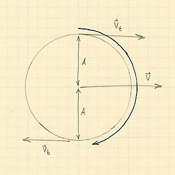
Let's start by examining a constituent of a water wave—a single water molecule—and then generalize to a whole wave. From the diagram we have a circle (which parameterizes harmonic motion) with radius $A$ and circumference $2 \pi A$. Invoking distance = rate × time, this leads to $v_\text{w} = 2 \pi A / T$, with $T$ equal to the rotational period of the circle. Now connect this to wavelength by recalling $T = 1 / f$ and $v = f \lambda$ to give $v_\text{w} = 2 \pi A v / \lambda$.
Referring to the diagram again, the velocities relative to $\mathbf{v}$ are
| $\displaystyle{ v_\text{t} = v - v_\text{w} = v \left( 1 - \frac{2 \pi A}{\lambda} \right) }$ | (3. |
for a point at the top of the circle, and
| $\displaystyle{ v_\text{b} = v + v_\text{w} = v \left( 1 + \frac{2 \pi A}{\lambda} \right) }$ | (3. |
for a point at the bottom of the circle.
At this point we will invoke Bernoulli's equation, which is conservation of energy applied to a dynamic fluid:
| $\displaystyle{ P_\text{t} + \frac{1}{2} \rho v_\text{t}^2 + \rho g y_\text{t} = P_\text{b} + \frac{1}{2} \rho v_\text{b}^2 + \rho g y_\text{b} \text{.} }$ | (3. |
In Equation (3.3) we will consider a small "hoop", or $P_\text{t} \simeq P_\text{b} \simeq$ atmospheric pressure. After some algebraic wizardry, we can approximate the speed of a deep-water wave:
| $\displaystyle{ \boxed{ v = \sqrt{\frac{g \lambda}{2 \pi}} \text{.} } }$ | (3. |